This article follows up on net2phone Canada's Google Sheet™ Add-On Beyond the Basics article, after you have built both (1) the inbound, and (2) the outbound pivot tables. Creating an impact table elevates the data so that information can be understood with new clarity. 

For simplicity, we recommend creating the impact table in the same spreadsheet as either the inbound or outbound pivot table. We will create this example in the Outbound sheet.

Step 1: Create Your Titles

Your titles should reflect the key metrics or conclusions you want to derive from the data. These will keep your table organized and focused on your goals.

For this example, our titles include:

• Outbound Total
• Inbound Total
• Outbound + Inbound
• Hours Worked
• % of Hours Worked
• Outbound Count
• Inbound Count

Step 2: Input Your Data 

We recommend inputting data from left to right to create a better flow and improve readability.

1. Leave 1-2 rows between your pivot table and the new table to make space for potential new columns.
   
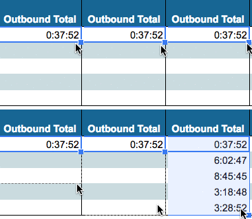
2. After entering the formula in the first cell, click and drag the corner to auto-fill the rest of the column.
   

Outbound Total

Calculate the total time (duration) a user has spent on outbound calls during the selected period.

Cell formula: =D#/86400

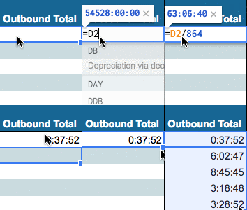
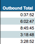
Convert seconds to minutes and hours: Format > Number > Duration. 

If you’re unfamiliar with this process, refer to our guide on How to Change Seconds to Minutes and Hours in Google Sheets™.

Inbound Total

Calculate the total time a user has spent on inbound calls.

Since the impact table is on the same sheet as the outbound pivot table, the formulas for outbound calls reference nearby Google Sheet^TM cells. The inbound pivot table is on a different sheet, so you'll need to manually link the data from that sheet to your impact table; this requires a few extra steps to transfer the inbound data.

Steps to input Inbound Total data:

1. Navigate to your Outbound pivot table and the impact table Google Sheet^TM.
2. In the first cell of the Inbound Total column, press the = key.
3. Switch to the Inbound Pivot sheet and click the first cell of the corresponding column.
4. Press Enter to lock the value.
5. Drag the formula down to auto-fill the remaining rows. 

Outbound + Inbound

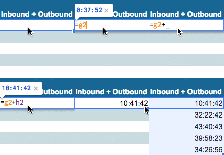
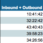
This column combines the outbound and inbound totals.

Cell formula:
=F# + H#

Hours Worked

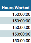
The total number of hours worked depends on the period of time covered by your pivot table and the daily working hours. In this example, we assume 7.5 hours per day over a 4-week period.

Formula for total hours worked:
7.5 x 5 = 37.5 (per week)
37.5 x 4 = 150 (total for the month)

% of Hours Worked

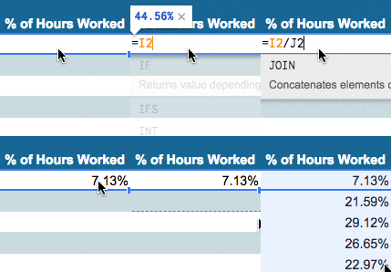
This column shows the percentage of time spent on calls, based on total hours worked.

Formula:
=I# / J# (inbound + outbound / total hours worked)

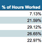
Format this as a percentage: Format > Number > Percent.
 

Outbound Count

This is the number of outbound calls made. Use the Start Time from the outbound pivot table.

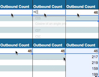
Formula:
=C#

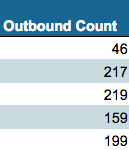
Inbound Count

This is the number of inbound calls received. Use the Start Time from the inbound pivot table.

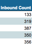
Follow the same steps as in the Inbound Total section to add this data.

Step 3: Identify Key Performance Indicators 

Refining data using impact tables helps you understand call center and agent performance, both individually and as a whole. You can copy and paste your impact table to a new sheet if needed. Tracking these metrics allows for deeper insights into agent performance, providing concrete data for promotions or bonuses.